Rendering check: math, code, and images

A first post that exercises a display equation, a Python code block, and an embedded image — so you can confirm the whole pipeline renders.

This post exists to verify that the three things I care about render correctly: LaTeX math, syntax-highlighted Python, and embedded images.

Math

Inline math works like y = \sigma(Wx + b), and display equations get their own centered block. Here’s the softmax used for classification over K classes:

\operatorname{softmax}(z)_i = \frac{e^{z_i}}{\sum_{j=1}^{K} e^{z_j}} \qquad \text{for } i = 1, \dots, K.

And the cross-entropy loss for a one-hot target y:

\mathcal{L}(y, \hat{y}) = -\sum_{i=1}^{K} y_i \log \hat{y}_i.

Code

The cell below is executed at render time and its output is embedded below it. Execution happens on my machine and the result is cached into _freeze/ (so CI never runs Python). A copy button appears on hover.

import numpy as np


def softmax(z):
    z = z - z.max()  # subtract max for numerical stability
    e = np.exp(z)
    return e / e.sum()


logits = np.array([2.0, 1.0, 0.1])
probs = softmax(logits)
print("probabilities:", np.round(probs, 4))
print("sum:", probs.sum())

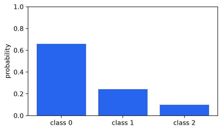
probabilities: [0.659  0.2424 0.0986]
sum: 1.0

Figures produced by code are captured too. Here we plot the softmax output:

import matplotlib.pyplot as plt

fig, ax = plt.subplots(figsize=(5, 3))
ax.bar([f"class {i}" for i in range(len(probs))], probs, color="#2563eb")
ax.set_ylabel("probability")
ax.set_ylim(0, 1)
plt.tight_layout()
plt.show()

Figure 1: Softmax probabilities for the logits above.

Images

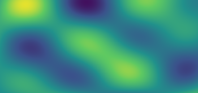
Below is an embedded raster image (a synthetic feature map). Figures get an automatic caption and can be clicked to enlarge.

Figure 2: A synthetic feature-map activation grid.

If the equation is centered, the code is colored with a copy button, and Figure 2 shows above with its caption — the pipeline works.