From HOG to DETR.

This is a blog post regarding object detection, spanning from the 2000s to modern times. Throughout the post, we will go through examples exploring how things got to where they are now. Note that this is not meant to describe every method in fine detail. It would take me a long time to write and draw visualizations for each problem, and second, it is not needed if it has already been written by the authors.

1 Introduction

Object detection is the task of taking an input image and, for every object of interest, both localizing it and classifying it. Localization can be as simple as a 2D bounding box, or as involved as a 3D box or a finer grained shape. We will stick to 2D examples.

Object detection is an old and well studied problem, with roots reaching back to the vision research of the 1970s and 80s (edge detectors, template matching, etc). Detection as we would recognize it today, though, arrived later: Viola–Jones in 2001 gave the first fast, practical face detector, and the HOG SVM pipeline in 2005 set the template for the classical era. Constrained by the limited compute and immature methods of the time, these early approaches were slow and, by today’s standards, quite inefficient.

Figure 1: Sliding window object detection (HOG + SVM).

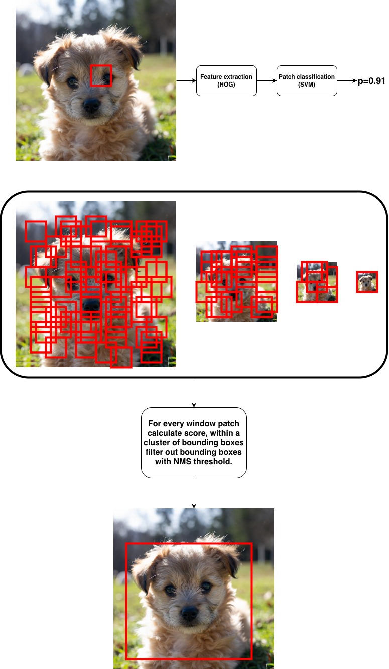
Not so long ago sliding window and continuously calculating features was the go to approach, it was intuitive but to today standards naive. Its principle is quite easy, across input image we would slide a predefined window with known size and calculate features from the window patch, later these features would be used to train a classifier to predict if there is an object of interest in the window patch. HOG + SVM pipeline from 2005 used this approach, we would calculate HOG features from window patch and based on them train an SVM classifier to predict if there is the object in the window patch. Note, that for every new object we have to train a new classifier.

This is also done at different scales as well, the window is slid across the image at each scale, features are computed for the pixels inside the window, and the classifier scores how likely it is that the object is present. Different scales are used so that we can pick up objects of different sizes, some closer to the camera and some further away. In practice this is usually done by keeping the window size fixed and rescaling the image into an image pyramid, rather than resizing the window itself. Then overlapping bounding boxes are pruned with non maximum suppression, and the highest scoring one is kept, which hopefully maps closely to the object in the image. So essentially we didn’t do any regression of bounding box coordinates, we just hoped that the predefined window would line up closely with the whole object at one of the pyramid scales. At this point you’re probably starting to sense that there must be a catch: it kinda works good for the dog image but how well does this scale to other use cases? The answer is, pretty bad.

1. As we can intuitively see, the whole process is computationally heavy: for every window position and every scale we have to compute features and run the classifier. And it only gets worse as the image grows, and new objects are introduced.

2. The approach relies on hand crafted features. Someone has to decide that HOG are the right thing to compute, so the features don’t come completely from the data. One big factor is the human’s intuition about what makes a dog look like a dog. Choose the wrong descriptor and the classifier has nothing useful to work with, and each new kind of object may call for a different hand tuned feature. This is exactly what deep learning later overturns: letting the network learn the features instead of prescribing them.

3. The pipeline trains one detector per object class. A single HOG + SVM answers “is there a dog here?” and nothing more. To handle a complex scene: a person in a room with a table, a bowl on it, apples and bananas inside you would need a separate trained detector for each object type, each run over the full image pyramid independently, and each with its own suitable window size and aspect ratio. A table is wide, an apple is small and round, a standing person is tall no single window shape fits them, and the cost multiplies with every class you add. Scenes with many objects at many scales are where the sliding window approach quietly falls apart.

Figure 2: (AI generated) A cluttered scene: many classes at many scales, each needing its own detector and window shape.

These problems push us to look for something smarter than per class search. It took a while after the mid 2000s for the next big thing to arrive, but sooner or later the 2010s reshaped object detection into the task as we practically know it today. Region proposal methods made their prominent debut in 2011 with Selective search, later published in the International Journal of Computer Vision in 2013.

2 Region proposals and Selective search

As the name suggests, we want an algorithm that proposes regions where our objects of interest might be located. So how do we do this? Do we need to train a model to find candidate regions, or without training, how then can we be confident the algorithm returns useful boxes? There are many ways to tackle this one of them is Selective search. In a nutshell, Selective search starts from image segmentation, merges regions by a similarity score until only one is left, and proposes the bounding boxes around those segments as candidate regions. The full procedure breaks down as follows:

1. Generate initial regions R with the Felzenszwalb segmentation method, setting the parameter k to, say, 100.

   1. This is an efficient graph based segmentation algorithm, used as a preprocessing step.
   2. k controls how easily pixels are grouped, a larger k gives larger segments in the final segmentation.

2. Compute the similarities between all pairs of neighbouring regions and put them in the similarity set S.

3. While S is not empty:

   1. Find the most similar pair s(r_i, r_j) in S.
   2. Merge r_i and r_j into a new region r_t.
   3. Remove from S all similarities involving r_i or r_j.
   4. Compute the similarities between r_t and its neighbours, and add them to S.
   5. Add r_t to R.

4. Repeat the whole procedure with increasing values of k (e.g. 100, 200, 300, …). A higher k gives a smaller number of segments at the start.

5. Draw bounding boxes around every region produced at every merge step, for every k.

6. Randomize/sort the boxes and remove near-duplicates.

7. Keep roughly the top 2000 boxes.

Great, now we have some region proposals. So what, are we going to compute HOG features and train the same SVM as before, just on nicer rectangles this time? Congratulations, we’d have reinvented the exact pipeline we were complaining about. Thankfully, new ideas aren’t slow, researchers came up with better ideas than HOG + SVM pipeline. One of the first real answers to this question came with the R-CNN paper.

3 R-CNN, Fast R-CNN and Faster R-CNN

Figure 3: R-CNN.

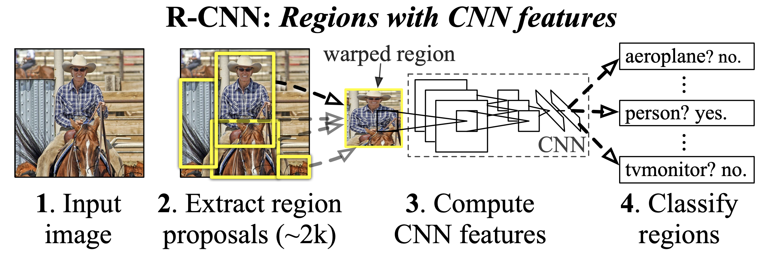
R-CNN arrived in 2014, and while it was one of the genuine breakthroughs in computer vision, the architecture came with a few… let’s call them challenges. You probably want to know what those challenges are. Patience first, the new stuff.

As you may have guessed from the name, we’re using convolutions. And the R at the front? It stands for Region, astonishing, I know. For the rest of the network architecture, all of its awkwardness I would suggest you to read the paper. It goes something like this: with Selective search find image patches, per class linear SVMs deciding whether the object of interest is in a given patch and separate bounding-box regressor refined the proposal coordinates.

Let’s take a step back. Sliding windows out, region proposals in; HOG out, CNN in. A couple of fundamental problems solved at the low, low price of running a full CNN forward pass on two thousand crops per image. What could possibly go wrong.

Well, this could go wrong:

1. The network processed each region proposal individually, which means the warped regions had to be processed one by one, and the resulting features had to be written to disk so they were ready as input for the SVMs. This was extremely storage heavy for the time, hundreds of gigabytes for a training set.

2. Training and inference are extremely slow because of the per-region processing. Inference took roughly 50 seconds per image with VGG16, and training took several days across its multiple stages.

3. Performance loss due to distorted regions. The authors called these warped regions, which was essentially an anisotropic resize of each proposal. This was necessary because AlexNet required a fixed 227 × 227 input.

Luckily Fast R-CNN came around the corner pretty fast in 2015, and solved these issues. It firsts computes features over the entire image, then use the region proposals to select the corresponding features from the last conv layer, and then RoI pooling converts each of those into a fixed 7 × 7 × 512 tensor so it can go into the fully connected layers for softmax classification and bounding box regression. The inference went from 50 seconds down to 2 seconds! The feature extraction approach has turned the Selective search algorithm to be the new bottleneck. A fast neural network was starved waiting for proposals, which lead to the next element that should be reinvented, the region proposal algorithm.

Figure 4: Fast R-CNN.

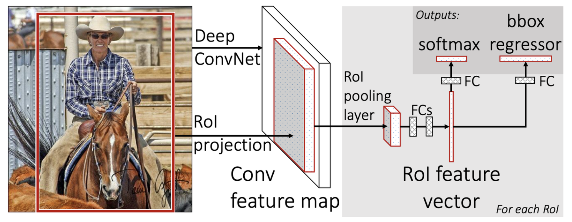
Couple of months later new paper, Faster R-CNN addressed these issues, by replacing the Selective search, CPU bound algorithm with a Region proposal neural network. This is the heart of the paper. The RPN is a small fully convolutional network that slides over the shared feature map and, at every location, predicts whether objects are present and roughly where. At each position on the feature map, the RPN places k reference boxes called anchors (typically 9: combinations of 3 scales × 3 aspect ratios). Anchors are fixed boxes of different shapes/sizes that act as starting templates.

For each anchor the RPN outputs:

• Objectness score (2 numbers): is this anchor object or background?
• Box refinement (4 numbers): adjustments to the anchor’s coordinates to better fit the object.

There’s a difference between how the computations are performed during training and at inference. When I first explored it, it didn’t make sense, it felt complicated. Looking at it today, it’s still complicated, and I never did come to like it. Anyway, training goes something like this:

• The image is passed through the VGG backbone, which outputs a 14 × 14 × 512 feature map. This output is shared by both the RPN and the second-stage detection head.

• Anchors are generated across the feature map (9 per cell, projected back onto the image) and labeled positive or negative by their IoU with the ground-truth boxes: ≥ 0.7 positive, ≤ 0.3 negative, in between ignored. Anchors crossing the image boundary are discarded.

• The RPN, a 3 × 3 conv followed by two sibling 1 × 1 convs runs over the feature map and predicts, for every anchor, 2 objectness scores and 4 box offsets.

• A mini-batch of 256 anchors is sampled from the labeled set, aiming for a 1:1 positive-to-negative ratio (padded with negatives if there aren’t enough positives). The RPN loss is computed on these 256 only.

• The RPN loss is the sum of a classification loss (binary cross-entropy over object vs. background) and a smooth L1 localization loss, the latter applied only to positive anchors.

L_{RPN}(p_i, t_i) = \frac{1}{N_{cls}} \sum_i L_{cls} (p_i, p_i^*) + \lambda \frac{1}{N_{reg}} \sum_i p_i^* L_{reg} (t_i, t_i^*)

where:

• i indexes anchors in the mini-batch,
• p_i ​is the predicted objectness probability and
• p_i^* is the ground-truth label (1 if positive, 0 if negative),
• t_i is the 4 predicted box offsets and
• t_i^* is the ground-truth offsets. ​

The p_i^* factor on the regression term is what restricts localization loss to positive anchors only. Classification term (binary, object vs. background):

L_{cls} (p_i, p_i^*) = - [p_i^* log p_i + (1 - p_i^*) log (1 - p_i)]

Regression term (smooth L1 over the 4 box coordinates):

L_{reg} (t_i, t_i^*)= \sum_{j \in \{x, y, w, h\}} smooth_{L1} \ \ (t_{ij} - t_{ij}^*)

Box parameterization (the offsets 𝑡 t are normalized relative to the anchor, not raw coordinates):

t_x = \frac{x-x_a}{w_a}, \quad t_y = \frac{y-y_a}{h_a}, t_w = log(\frac{w}{w_a}), t_h = log(\frac{h}{h_a})

• Separately, the RPN’s predicted offsets are applied to all anchors to produce proposal boxes. These are ranked by objectness, pruned with NMS (IoU 0.7), and the top M are kept. From these, 256 proposals are sampled for the second stage — 25% positives (IoU ≥ 0.5 with a ground-truth box) and the rest negatives.

• These proposals, together with the VGG feature map, go to ROI pooling and then to the FC layers for object classification and class-specific bounding-box regression.

• The outputs are compared to the ground truth: cross-entropy over K + 1 classes plus smooth L1 on the boxes (positives only). Aggregated, this is the detection loss.

L_{det} (p, u, t^u, v) = L_{cls} (p, u) + \lambda [u \ge 1] L_{reg} (y^u, v)

where:

• p is the softmax distribution over K + 1 classes,
• u the ground truth class,
• t^u the box offsets for the predicted class u,
• v the ground truth offsets.

The Iverson bracket [u \ge 1] zeroes the box loss for background proposals (u=0), the multi class analogue of the p_i^* factor above. Classification here is cross-entropy over K+1 classes:

L_{cls} (p, u) = - log(p_u)

• The detection loss and the RPN loss are summed into the final loss.

L = L_{RPN} + L_{det}

• Both losses backpropagate into the shared backbone. The RPN loss updates the RPN head and the backbone; the detection loss updates the detection heads and the backbone. Gradients are not passed back through the proposal coordinates the proposals are treated as fixed inputs to ROI pooling.

Luckily, inference is easier:

• The image is passed through the VGG backbone to get the feature map,

• RPN predicts objectness scores and box offsets for every anchor,

• The offsets are applied to the anchors to produce proposals, which are ranked by objectness, pruned with NMS (IoU 0.7), and cut to the top M (~300).

• These proposals, together with the feature map, go to RoI pooling and then to the FC layers, which output class scores and class-specific box offsets.

• The offsets are applied to the proposals, low-scoring boxes are thresholded away, and a final per-class NMS removes duplicates.

That was intense, but we made it through. We skipped the finer details of R-CNN and Fast R-CNN and instead took a small detour through Faster R-CNN. Even from that one example, you can see how quickly a neural network architecture can get messy: the sampling here, the stop gradient there, two different mini batches with two different ratios, a loss stitched together from four pieces. Honestly, the architecture side when we connect together blocks and layers like Lego bricks is the fun part, because you let your imagination out. The harder discipline comes when you design the actual loss function, the thing that has to teach the network something useful. Wrapping everything up, that’s where intuition alone stops being enough and you need a real understanding of how each piece behaves and how they fit together.

4 YOLO

YOLO (You Only Look Once) is a CNN-based object detection algorithm introduced in 2015. One natural way to think about detecting objects is to lean on time: if you have a stream of video frames, you can watch how the scene evolves and use several past frames to help decide what’s in the current one. This makes intuitive sense as motion and continuity carry a lot of information, and a fuzzy object in one frame often becomes obvious once you’ve seen the few frames leading up to it.

The catch is that this kind of temporal approach asks for more of everything:

1. more data, since you need sequences rather than single images

2. more compute, since you’re processing several frames to make one decision

3. and more complexity, since the model has to carry information across time.

It’s powerful, but heavy. As you can relate, it’s often easier and faster to judge what you’re looking at right now than to reconstruct a story from what happened moments before. The researchers behind YOLO built a method that needs only a single still image to detect all the objects in it, without relying on any past frames at all. That’s exactly what the name captures: the model looks once and predicts everything. This turned out to be a big deal, YOLO over the years of development stayed light enough to run in real time, which made object detection available for applications on edge devices. Today latest YOLO models make it possible to run object detections with speeds over 100FPS on edge devices like a Jetson.

Researching the YOLO model has become quite a hassle, since by now there are over ten versions, each introducing something new, removing an older part, and so on. One could probably write a whole book on how things have changed over the past years, which makes it hard to decide where to even start. At the time of writing, the latest release is YOLOv26, which, if we’re being honest, doesn’t share many architectural similarities with the very first version. For that reason, I’ll briefly go over the latest version and point out its most important parts. Anyone interested in the historical changes can read the corresponding papers.

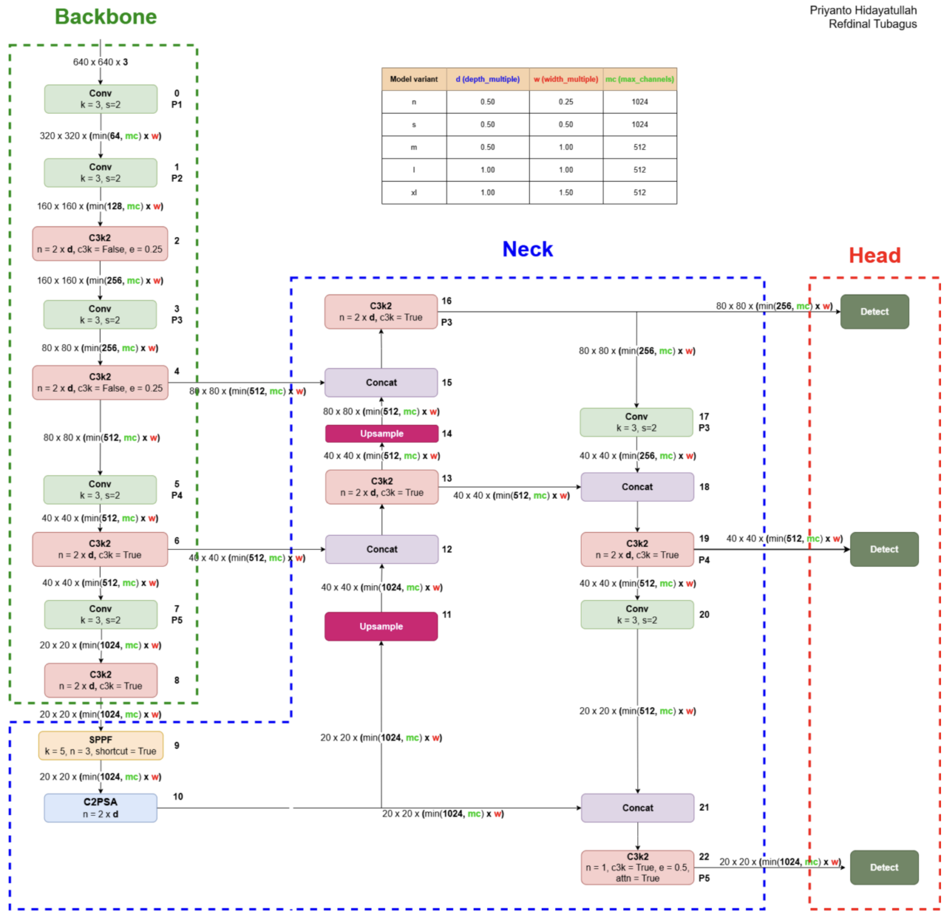
Figure 5: YOLO architecture: backbone, neck, and detection head (diagram by Priyanto Hidayatullah and Refdinal Tubagus).

YOLO26 follows what is, by today’s standards, a classical architecture for object detection. The network is built from three parts:

1. Backbone — Computes features from the input image at different scales. Usually a CNN, such as a ResNet. YOLO uses its own CSP style design, not literally ResNet.

2. Neck — Takes the backbone features and processes them further, applying some sort of interaction and fusion of feature maps across different scales.

3. Detection head — Uses the neck’s output to produce the detections: classification scores for each label and bounding boxes.

When you first look at the block diagram, without any knowledge of the current research state, it can be intimidating. But the backbone is a CNN, the neck (PAN-FPN) is also convolution-based, and the detection head is CNN-based too, with a few add-ons. So chill, it’s just convolution, not nuclear physics.

One could arguably say that Faster R-CNN follows same approach: backbone, neck head. But we will leave that for a different post, for now and YOLO this is mainly it, I will make overviews of these elements in other blocks an link the accordingly here, for now we passed YOLO model.

5 Transformer architecture

5.1 Introduction

The transformer architecture was actually introduced to the deep learning field years before the famous paper came out. At the beginning it wasn’t a big deal, later, in 2017, with the paper “Attention Is All You Need” for NLP tasks, it became the next big thing. What’s interesting is that the attention mechanism itself was already known, but nobody was aware of how powerful it was.

I don’t have this second hand: one of the paper’s authors told this story at a conference I attended. According to them, the effectiveness of the approach was found partly by luck, through an ablation study where they stumbled onto a surprising result. As I recall the telling, they had been working on a completely different architecture a highly complex, well established one and had run tons of experiments on it: adding new layers and components, tweaking hyperparameters, trying to squeeze something better out of it and push past the state of the art. Eventually they got there, and were ready to write up the work.

Then, out of nowhere, a researcher who was experimenting with the model wondered what would happen if he simply took couple of layers out. The logical expectation was that the model would be smaller, with fewer parameters, and therefore worse than the one they had spent months developing. Instead, the stripped down version performed astonishingly well, better than everything they had built up to that point. So they kept cutting the architecture down, piece by piece, until all that was left was the attention mechanism. At that point they realized attention was all they needed, and named the paper accordingly.

5.2 Attention is all you need

Way before this conference, when I was first researching attention, I came across the usual explanation based on query, key, and value matrices. The story went something like: the query is what you’re asking for, the key is what you match against to find it, and the value is what you get back. I may not have the wording exactly as it’s usually told, but you get the idea, and it’s awful. Not a single word about embedding spaces, about representing elements mathematically, or about how to actually compute the relationships between them. I was lost in endless abstractions. So before we get to the transformer architecture, let’s take a look at how we can represent something with numbers in the first place. Let’s assume we have the sentence:

• “The king and queen ruled the mighty lion.”

and want to understand the underlying connections between its words. What we usually do first is embed each word into an embedding space, so that each one is represented as a numerical vector. (Note: in NLP there is a concept called a token, and it’s actually the token that gets embedded, not necessarily the whole word but for our purposes we’ll skip that and treat words as tokens.) So instead of viewing the sentence as a set of words, we now have a numerical representation of them in a high dimensional space, one that can potentially hold many complex relationships between them. Embedding spaces can go from a low 2D space to thousands of dimensions, and there is no strict upper limit or ceiling on how many dimensions you can use. Now, back to assessing connectivity: because the elements are now numerical vectors, we can do all sorts of things with them and for connectivity specifically, we can compute a similarity score that tells us how close together or far apart they lie.

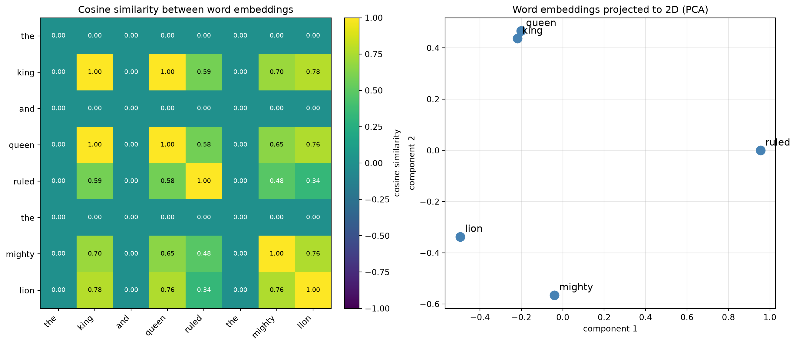
The two figures below show this in action. On the left is a cosine similarity heatmap: every cell is the similarity between one pair of words, running from −1 (opposite) through 0 (unrelated) to 1 (highly similar). The bright diagonal is each word compared with itself (always 1), and the interesting signal is off the diagonal king and queen score highly because their vectors point in nearly the same direction, while the function words “the” and “and” stay dark against everything, since their near zero vectors have no meaningful direction to align with. On the right, the same vectors are projected down from their original dimensions to 2D with PCA, so we can actually see them as points. Words with similar meaning land close together king and queen sit almost on top of each other, lion is nearby along the “power” direction but pulled away for being an animal rather than royalty, and mighty floats between them.

After the example we have hopefully got an intuition what an embedding space is, how can an element be projected that is represented in that space and how can it relate to other elements. Lets go forward with the transformer architecture. The transformer consists of an encoder and a decoder. Given an input sequence, the encoder produces a continuous representation, from which the decoder generates an output sequence. The decoder is autoregressive, which means it consumes the previously generated symbols as additional input when producing the next output. As the image shows, the encoder and decoder mainly consist of self-attention and fully connected layers.

Figure 6: Transformer architecture.

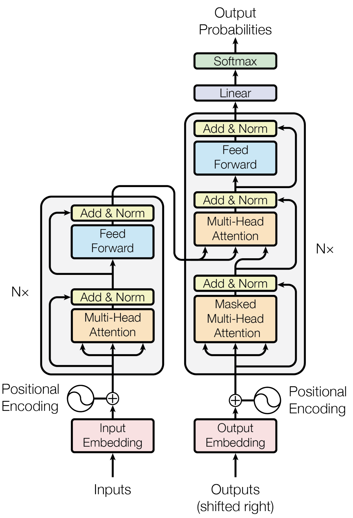
Self-attention is an attention mechanism that relates different positions of a sequence in order to compute a representation of that sequence. In other words, it lets us express mathematically how the elements of a sequence relate to one another. Oh, we have actually seen this problem idea in our king, queen and lion example. How is this done here? Well, actually the same way. If we can represent each element with a numerical form such as a vector, and can compute the similarity between those vectors then we can analyze the relationships between embedded, high dimensional data. There are many metrics for measuring it, and cosine similarity is one of them. Cosine similarity measures how aligned two vectors are by taking the cosine of the angle between them, producing a score from −1 to 1: values closer to 1 mean high directional similarity, 0 means orthogonal, and −1 means opposite.

\cos(\theta) = \frac{A \cdot B}{\lVert A \rVert \, \lVert B \rVert} = \frac{\displaystyle\sum_{i=1}^{n} A_i B_i} {\displaystyle\sqrt{\sum_{i=1}^{n} A_i^2}\,\sqrt{\sum_{i=1}^{n} B_i^2}}

When looking at an entire sentence, raw values between -1 and 1 for word-to-word relationships makes it difficult to interpret exact connectivity. A better approach is to use weights that sum up to 1. To achieve this, we can apply the softmax function to the cosine similarity outputs and then multiply the resulting weights by the word embeddings.

Self-attention is related to cosine similarity, but with an important difference. Cosine similarity divides the dot product by both vectors lengths, removing magnitude entirely. Attention doesn’t do that, it keeps the raw dot product and divides only by a single constant, d_k, based on the vector dimensionality. That constant isn’t there to normalize magnitude it’s there to keep the dot products from growing too large as the dimension increases, which would otherwise make the softmax gradients vanish.

Attention \ weight = \frac{Q \cdot K^T}{\sqrt{d_k}}

Note that many people get confused here, thinking this is the attention score but it isn’t. To get there, this first has to pass through a softmax, and then a final matrix multiplication with the value matrix V.

Attention(Q, K, V) = softmax \left( \frac{Q \cdot K^T}{\sqrt{d_k}} \right) V

Okay, hopefully the dot product and the division make sense so far. But you’re probably now asking: what’s the point of these weights, what are those matrices Q, K, V and why has this suddenly gotten more complicated than our easy example? If that’s where you are right now, good that’s exactly where you should be. Many people were stuck at this same spot before you, and it’s the moment right before it clicks. Let’s connect the two versions we’ve seen.

In our easy example, there were no trainable weights at all. We simply took the sequence elements, computed raw embeddings, and computed dot products between them to see how much each element should attend to the others. Then we used those scores directly to build a weighted sum of the same embeddings. That was enough to build intuition, but a real model needs to learn, and you can’t learn anything if there’s nothing to adjust. That’s what the trainable weights are for and the actual answer to your question “what’s the point of these Q, K, V matrices”. Instead of using the embeddings directly, we now multiply each embedding by three separate learned weight matrices to produce three different vectors for every token: a query, a key, and a value. They use the same embedding, but because each matrix is different, they project that embedding into three different roles. The query and key are not the same thing, they’re two different views of the same original token. So when we say tokens query, key or values we mean the output that we get when we multiply its embeddings with that query, key or value matrix.

Now the mechanism runs in three clean steps:

1. Attention scores. For each token, we take its query and compute a dot product against the key of every token in the sequence (including itself). This gives us raw scores that measure how relevant every other token is to the current one.

2. Attention weights. We divide those scores by the square root of the key dimension, this keeps the numbers in a stable range so the next step behaves well and pass them through a softmax. Now we have the attention weights: values that sum to 1 and tell us how much focus each token receives.

3. Context vector. Finally, we multiply the attention weights by the value vectors and sum them. This weighted sum is the context vector, the output that stores, for each token, the important context gathered from itself and from every other token it attended to.

In the easy example, the final weighted sum was over the raw embeddings themselves the tokens could only pass along their original representation. Now, that sum is over the value vectors, which are learned transformations of those embeddings. In other words, the value matrix lets each token decide what information to actually contribute once it’s been attended to, rather than just handing over its raw embedding. That’s the difference between a fixed mechanism and one that can learn.

5.3 Vision Transformer

Now back to vision. In late 2020, a team at Google published an adaptation of the transformer for vision tasks: “An Image is Worth 16×16 Words: Transformers for Image Recognition at Scale.” Adapting the transformer to images wasn’t trivial, mainly because of the computational cost it brings. From the attention equations you can see that the cost grows with the length of the input sequence and the culprit is the dot product between the query and key matrices, which scales quadratically with the number of tokens. So if you naively treat every pixel as a token, things get ugly fast: for a modest image the sequence length explodes, and the attention computation becomes hopelessly expensive. To get around this, the Google team took a simple but effective step: instead of treating each pixel as a token, they split the image into fixed-size patches (16×16 pixels each) and treated every patch as a token. This cuts the sequence length dramatically a 224×224 image becomes just 196 patches instead of over 50,000 pixels. Straightforward as this sounds, getting it to actually work well was another matter, and much of the paper is about what it takes to make it pay off. The pipeline works like this. Each patch is flattened into a vector and passed through a linear projection into an embedding space. A learnable positional embedding is added to each patch embedding so the model retains some sense of where each patch sat in the original image information that would otherwise be lost once the grid is broken into a flat sequence. This sequence is then fed to a standard transformer encoder, where multi-head self-attention lets every patch attend to every other patch, mixing in global context across the whole image.

There’s one more important ingredient. Borrowing a trick from BERT, the authors prepend an extra learnable embedding to the sequence, the class token which carries no patch content of its own. As the sequence passes through the encoder, this token attends to all the patches and accumulates a global summary of the image. At the output, its final representation is the only one sent to the MLP head, which produces the class prediction. Because the encoder’s whole job is to share information between embeddings via attention, the class token ends up being a natural place to gather the global context the classifier needs.

Figure 7: Transformer adaptation to vision by Google.

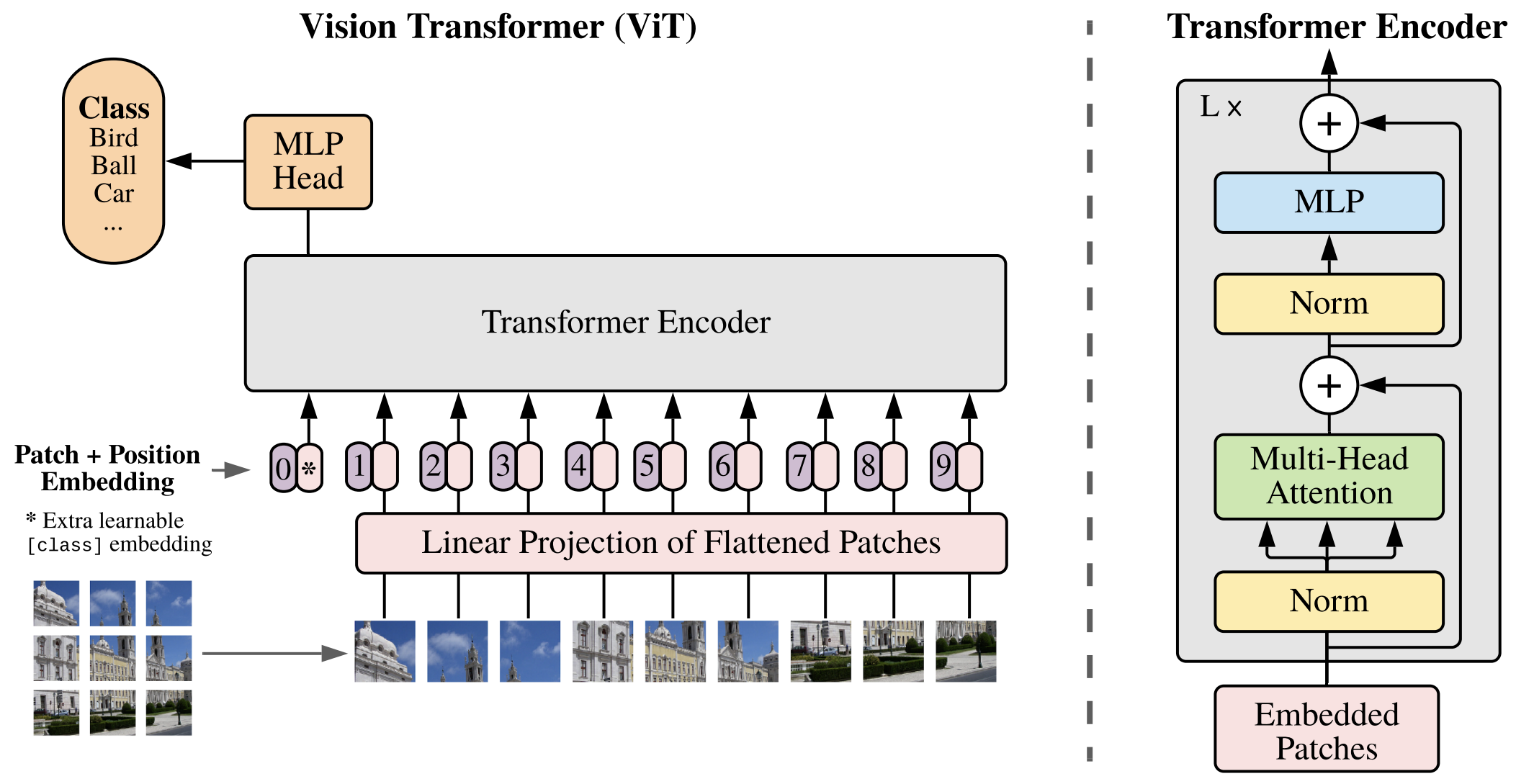
The loss function is Softmax cross-entropy over C classes with label smoothing.

L = - \sum_{i=1}^C y_i^{LS} log (p_i) = -(1-\epsilon) log (p_c) - \frac{\epsilon}{C-1} \sum_{i \ne c} log (p_i)

y_i^{\text{LS}} = \begin{cases} 1 - \varepsilon & \text{if } i = c \\ \dfrac{\varepsilon}{C - 1} & \text{otherwise} \end{cases}

The one-hot target is softened by a factor \epsilon, spreading a little probability mass onto the wrong classes. So the correct class is no longer pushed toward probability 1, and the wrong classes aren’t pushed fully to 0. This discourages the network from becoming overconfident and tends to improve generalization and calibration. Classification with the ViT approach seems easy, what about detection?

6 DETR

We came a long way from old sliding windows over CNN architectures to detection transformers. Why detection transformers at all? Well, they did remarkably well in NLP, and in image classification, so why don’t we try them in object detection? DETR came out in 2020 as a result of work from Facebook’s research group. At that time object detection was ruled mainly by Faster R-CNN and YOLO models, which had some caveats. First is that they used anchor boxes, and defining these requires knowledge about our particular problem the shape of the objects, size and so on. Second, the computational speed of these methods was heavily affected by NMS. To simplify this, DETR proposes an end-to-end approach where the model produces a direct set of predictions, bypassing any postprocessing steps.

On its own the DETR architecture is straightforward: a CNN backbone for feature extraction, a transformer encoder-decoder, and a feed-forward network (FFN) for final detection predictions. Yep, you see right, now for object detection we are using also the decoder.

Backbone. Starting from an input RGB image x_{\text{img}} \in \mathbb{R}^{3 \times H_0 \times W_0}, the backbone generates a feature map f \in \mathbb{R}^{C \times H \times W}, where C = 2048, H = \frac{H_0}{32}, and W = \frac{W_0}{32}.

So first we train a ResNet for image recognition task, then we cut the recognition head off and flatten out the output so we can input it to the encoder.

Transformer encoder. A 1 \times 1 convolution first reduces the channel dimension of the backbone feature map from C to d. Since the encoder expects a sequence, the resulting map is flattened to a d \times HW tensor. A fixed 2D sine positional encoding is added it is not learned in the default setup and the result is passed to the Transformer encoder. Note that this encoding is added to the queries and keys at every encoder layer, not only once at the input. Each encoder layer follows a standard architecture: multi-head self-attention followed by a feed-forward network. BTW, the encoder there is to output the embedded vector d \times HW with enriched global context information, so it’s some sort of a feature interaction i.e. propagation of information in the image from one part to another.

Transformer decoder. The decoder uses encoder embeddings information to enrich N learnable object queries of size d using multi-head self-attention and encoder-decoder attention (cross attention). BTW, these object queries at beginning don’t store any information, they are randomly initialized. Each decoder layer first does self-attention among the queries, then cross-attention into the encoder output. The object queries are decoded independently into box coordinates and class labels by the FFN.

Prediction FFN. The final prediction is computed by a 3-layer perceptron with ReLU activations and hidden dimension d, followed by a linear projection. The FFN predicts the normalized center coordinates, height, and width of each bounding box relative to the input image. A softmax layer predicts the class label. Since we always predict a fixed set of N boxes typically much larger than the actual number of objects in an image a special class label \varnothing is used to indicate “no object detected.” This plays a similar role to the background class in standard object detection pipelines.

Figure 8: DETR by Facebook.

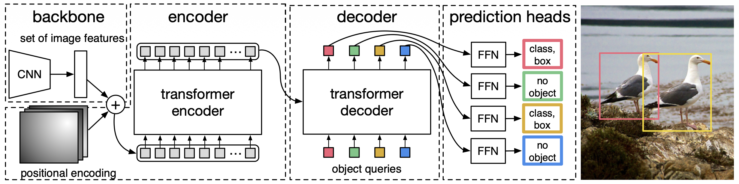
The decoder produces a fixed-size output of N predictions, which is usually much larger than the actual number of objects in the image. The loss function performs bipartite matching between predictions and ground truth, then optimizes object-specific losses. Let y denote the ground truth set of objects and \hat{y} = \{\hat{y}_i\}_{i=1}^N the set of N predictions. Since N is larger than the number of ground truth objects, y is padded with \varnothing (no object) to match size N.

Each ground truth element can be written as y_i = (c_i, b_i), where c_i is the target class label and b_i \in [0,1]^4 is the target bounding box. For a prediction with index \sigma(i), we define \hat{p}_{\sigma(i)}(c_i) as the predicted probability of class c_i and \hat{b}_{\sigma(i)} as the predicted bounding box.

Matching cost:

L_{\text{match}}(y_i, \hat{y}_{\sigma_i}) = -\hat{p}_{\sigma(i)}(c_i) + L_{\text{box}}(b_i, \hat{b}_{\sigma(i)})

To find the optimal bipartite matching, we search over all permutations for the assignment with lowest total cost:

\hat{\sigma} = \underset{\sigma}{\arg\min} \sum_{i=1}^N L_{\text{match}}(y_i, \hat{y}_{\sigma(i)})

Hungarian loss:

L_{\text{Hungarian}}(y, \hat{y}) = \sum_{i=1}^N \left[ -\log \hat{p}_{\hat{\sigma}(i)}(c_i) + L_{\text{box}}(b_i, \hat{b}_{\hat{\sigma}(i)}) \right]

Bounding box loss: L_{\text{box}} is a linear combination of L1 loss and generalized IoU (GIoU) loss, making it scale-invariant.

7 Deformable DETR

Deformable DETR borrows the central idea introduced by deformable convolutions: adaptive, learned sampling instead of fixed sampling. To see why that’s good, it helps to take a closer look at the deformable convolution itself.

7.1 Deformable convolution

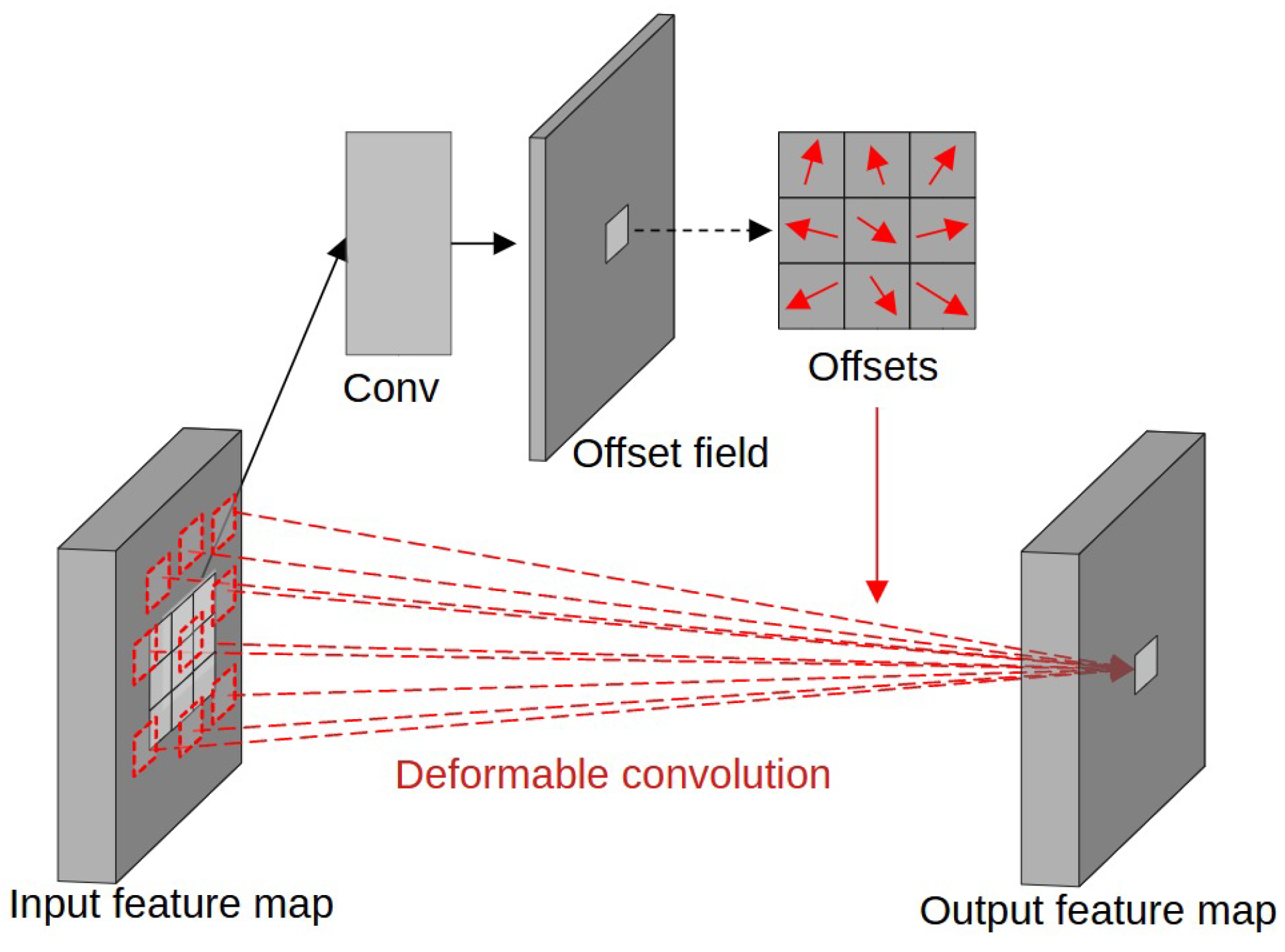
A standard convolution with kernel size k takes a k \times k block of pixels in a fixed square arrangement and computes the convolution over them. All the pixels used are immediate neighbours on a rigid grid. This isn’t always the most effective choice many objects have shapes that don’t fit neatly into a square. So deformable convolution learns offsets between the regular sampling positions and the locations it actually samples from. In effect, it learns where to look, choosing sampling locations that may suit the underlying object better than a rigid grid would. The sampling locations become

p + p_k + \Delta p_k

where:

• p is the center pixel
• p_k is the regular kernel offset
• \Delta p_k is the learned kernel offset.

So basically you let the network reshape its own sampling pattern for the specific input, rather than forcing every feature to be computed from a fixed square. For the cost of a few extra parameters a small side branch that predicts the offsets you get a kernel that adapts its geometry to the content. The name “deformable” comes from the fact that the convolution is no longer locked to a rigid grid shape but can deform to follow the object.

Figure 9: Deformable convolution.

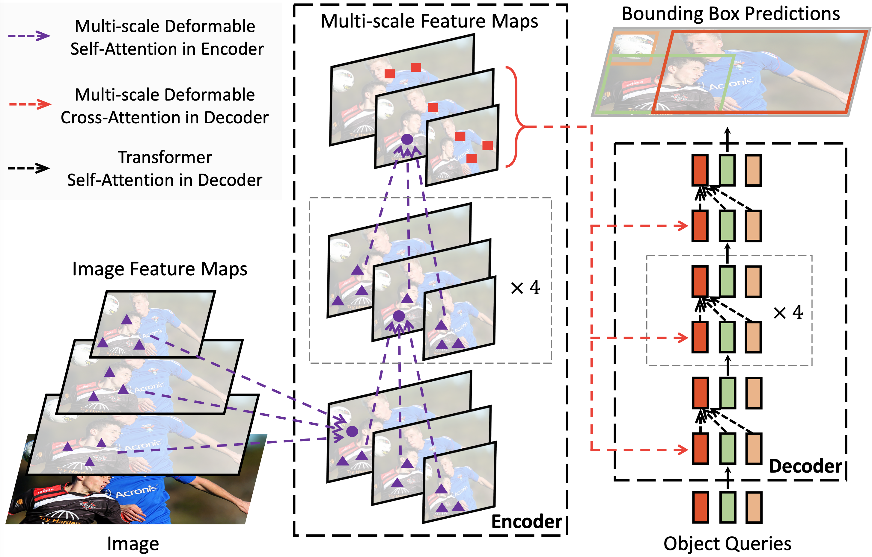
In the same way, Deformable DETR doesn’t compute attention from each query to every spatial location only to a small set of learned sampling points. This sharply reduces the cost of the attention operation. Second, it uses multiscale features, without an FPN by extending deformable attention module for multi-scale feature maps. This further improves the detection of small objects significantly. Third, the decoder doesn’t predict the bounding boxes directly, rather each decoder layer iterative refines the bounding boxes. All of this affect the accuracy and convergence speed 10x of deformable DETR compared to DETR.

Even after all these modifications, Deformable DETR isn’t quite the algorithm that would be used on edge devices, it is still too slow.

Figure 10: Deformable DETR.

8 Real time DETR

The DETR architecture was a great step forward in object detection with transformers, but it was rarely used in production. Nevertheless it was enormously influential and produced whole DETR family of models. The caveats were:

1. Training was slow, especially the multi-head self-attention mechanisms in the encoder part. Long training epochs are necessary for the attention weights to be learned to focus on sparse meaningful locations. The attention weights computation in encoder is of quadratic computation with respect to pixel numbers. Also decoder object queries took a long time to get somewhere. Thus, it is of very high computational and memory complexities to process high-resolution feature maps.

2. Because of the high complexity to process high-resolution feature maps DETR has relatively low performance at detecting small objects. Modern object detectors usually exploit multi scale features, where small objects are detected from high resolution feature maps.

3. Inference was awful compared to YOLO models or Faster R-CNN, this method didn’t stand a chance.

So even though it got rid of some post-processing steps, DETR was far from being useful in industrial settings. This pushed research in the direction of producing new lightweight models.

8.1 RT-DETR

RT-DETR is one of the successors of DETR, developed to build a real-time object-detection transformer that runs fast without sacrificing accuracy. To that end, the architecture borrows ideas from DETR, Deformable DETR, and other detection networks, with some additions:

• Backbone: ResNet or PP-HGNetV2 (HGNetV2), both conv-based. It takes the last three stages S3, S4, S5 for multi-scale feature interaction.

• Efficient Hybrid Encoder (AIFI + CCFF): the main contribution. It removes the expensive full self-attention over all scales and replaces it with intra-scale interaction (AIFI) plus cross-scale fusion (CCFF).

  • AIFI: self-attention applied only to S5, the deepest and most semantic feature map. The rationale: deep features benefit most from global self-attention, while applying it to shallower maps (S3, S4) is expensive and adds little, since those carry local detail rather than long-range relationships.

  • CCFF: fuses S3 and S4 (raw, not attention-processed) with AIFI’s output (the attention-processed S5), using a CNN-based, PAN-like top-down/bottom-up fusion path.

• IoU-aware Query Selection: rather than using a fixed set of learned queries, the encoder scores its output features and selects the most promising ones to initialize the decoder queries. The “IoU-aware” part means the selection is trained so that the classification confidence correlates with localization quality the model prefers features that are both confidently classified and well-localized.

• Transformer Decoder and Detection heads: a DETR-style decoder self-attention among queries plus cross-attention into the encoder memory. The cross-attention is deformable, so each query samples a small fixed number of points near its current reference box across the multi-scale maps rather than attending densely to everything, which keeps decoding cheap. Each decoder layer iteratively refines its reference boxes for the next layer.

From these points and knowing how vanilla DETR and Deformable DETR work we can see where the authors focused. Dense self-attention over all feature maps is replaced by a custom encoder that runs self-attention only on the smallest, most semantic map and uses convolutional fusion for the rest. Queries are selected by a scoring mechanism, saving work in the decoder’s cross-attention. The decoder layers then perform deformable cross-attention and iteratively refine the boxes. In short: take the prior work and squeeze it while holding as much accuracy as possible while pushing inference time as low as it will go.

There’s a lot of work on this topic. And by “a lot,” I mean there are four separate papers just for the RT-DETR line: RT-DETR, RT-DETRv2, RT-DETRv3, and RT-DETRv4. Other researchers have added to the topic also: D-FINE based on RT-DETR reworked the iterative bounding box regression, DEIM introduced a new loss that improves convergence, and then there’s RF-DETR, LW-DETR, and others. We’re not going to march through every one of them, by the time I finish some, there’d be three more waiting. Machine learning moves fast, and object detection with DETRs is a tiny corner of it. So consider this your jumping off point, and keep yourself updated at your own pace.

9 Conclusion

This was quite a read. When I first started exploring the topic, I searched for resources with LLMs, and it blew up fast. Research papers and GitHub repos gave me something to work with quickly, but the gaps in my understanding how things actually work and fit together soon became hard to ignore. So I started reading the papers properly and keeping my own notes in Obsidian, and at some point I thought: why not turn these into a blog? They didn’t look that bad, I figured. They were bad, next to an actual post, my notes read like a ransom letter. Never mind that, though! For me, this blog post is a good introduction to the current state of object detection. One could probably argue that I missed some important stuff, and I probably have, but this is already too long, so I’ll finish here. Nobody knows everything, and there will always be something new. These sentences are already becoming my past, let’s see how long they remain relevant.

Bonus storyline, the hidden motivation. Machine learning engineering in the age of foundation models has become heavily deployment focused. A lot of gluing things together, and precious little time for building anything from scratch. LLMs made everything move faster. Ten years ago, writing, understanding, and actually shipping a hundred lines of code was a real accomplishment. Today people assemble entire products by asking nicely and hoping. Sometimes it works. Sometimes you overengineer to a problem nobody had. And sooner or later you hit the wall where your Claude or Codex friend starts confidently inventing stuff that doesn’t exist and you find yourself going in circles chasing a fix that would’ve been obvious if you understood how any of it worked underneath.

Don’t misread me: as an engineer you should lean on these tools iterate fast, look things up, don’t waste an afternoon losing a knife fight with a semicolon. But you should never let them inflate your knowledge. In finance, inflation is the loss of money’s buying power: a dollar a year ago bought more than it does today. Leave your money in the bank and it quietly rots, invest it in something that grows and you protect your net worth. Knowledge is no different. Coast on borrowed answers and your understanding devalues while you’re not looking and the job market doesn’t care that your agent wrote it. Invest your time in genuinely learning the fundamentals and the new developments in your field, and it compounds. The punchline is the part people miss: the better you actually understand this stuff, the more you get out of the tools, not less. The people who’ll be replaced by AI aren’t the ones who learned the fundamentals they’re the ones who thought they could skip them.

References

Bahdanau, Dzmitry, Kyunghyun Cho, and Yoshua Bengio. 2015. “Neural Machine Translation by Jointly Learning to Align and Translate.” International Conference on Learning Representations (ICLR). https://arxiv.org/abs/1409.0473.
Carion, Nicolas, Francisco Massa, Gabriel Synnaeve, Nicolas Usunier, Alexander Kirillov, and Sergey Zagoruyko. 2020. “End-to-End Object Detection with Transformers.” European Conference on Computer Vision (ECCV). https://arxiv.org/abs/2005.12872.
Chen, Qiang, Xiangbo Su, Xinyu Zhang, et al. 2024. LW-DETR: A Transformer Replacement to YOLO for Real-Time Detection. https://arxiv.org/abs/2406.03459.
Dai, Jifeng, Haozhi Qi, Yuwen Xiong, et al. 2017. “Deformable Convolutional Networks.” Proceedings of the IEEE International Conference on Computer Vision (ICCV). https://arxiv.org/abs/1703.06211.
Dalal, Navneet, and Bill Triggs. 2005. “Histograms of Oriented Gradients for Human Detection.” Proceedings of the IEEE Conference on Computer Vision and Pattern Recognition (CVPR), 886–93.
Devlin, Jacob, Ming-Wei Chang, Kenton Lee, and Kristina Toutanova. 2019. “BERT: Pre-Training of Deep Bidirectional Transformers for Language Understanding.” Proceedings of the Conference of the North American Chapter of the Association for Computational Linguistics (NAACL). https://arxiv.org/abs/1810.04805.
Dosovitskiy, Alexey, Lucas Beyer, Alexander Kolesnikov, et al. 2021. “An Image Is Worth 16x16 Words: Transformers for Image Recognition at Scale.” International Conference on Learning Representations (ICLR). https://arxiv.org/abs/2010.11929.
Felzenszwalb, Pedro F., and Daniel P. Huttenlocher. 2004. “Efficient Graph-Based Image Segmentation.” International Journal of Computer Vision 59 (2): 167–81.
Girshick, Ross. 2015. “Fast R-CNN.” Proceedings of the IEEE International Conference on Computer Vision (ICCV). https://arxiv.org/abs/1504.08083.
Girshick, Ross, Jeff Donahue, Trevor Darrell, and Jitendra Malik. 2014. “Rich Feature Hierarchies for Accurate Object Detection and Semantic Segmentation.” Proceedings of the IEEE Conference on Computer Vision and Pattern Recognition (CVPR). https://arxiv.org/abs/1311.2524.
He, Kaiming, Xiangyu Zhang, Shaoqing Ren, and Jian Sun. 2016. “Deep Residual Learning for Image Recognition.” Proceedings of the IEEE Conference on Computer Vision and Pattern Recognition (CVPR). https://arxiv.org/abs/1512.03385.
Hidayatullah, Priyanto, and Refdinal Tubagus. 2026. YOLO26: A Comprehensive Architecture Overview and Key Improvements. https://arxiv.org/abs/2602.14582.
Huang, Shihua, Zhichao Lu, Xiaodong Cun, Yongjun Yu, Xiao Zhou, and Xi Shen. 2024. DEIM: DETR with Improved Matching for Fast Convergence. https://arxiv.org/abs/2412.04234.
Krizhevsky, Alex, Ilya Sutskever, and Geoffrey E. Hinton. 2012. “ImageNet Classification with Deep Convolutional Neural Networks.” Advances in Neural Information Processing Systems (NeurIPS), 1097–105.
Kuhn, Harold W. 1955. “The Hungarian Method for the Assignment Problem.” Naval Research Logistics Quarterly 2 (1–2): 83–97.
Liao, Zijun, Yian Zhao, Xin Shan, et al. 2025. RT-DETRv4: Painlessly Furthering Real-Time Object Detection with Vision Foundation Models. https://arxiv.org/abs/2510.25257.
Lin, Tsung-Yi, Piotr Dollár, Ross Girshick, Kaiming He, Bharath Hariharan, and Serge Belongie. 2017. “Feature Pyramid Networks for Object Detection.” Proceedings of the IEEE Conference on Computer Vision and Pattern Recognition (CVPR). https://arxiv.org/abs/1612.03144.
Liu, Shu, Lu Qi, Haifang Qin, Jianping Shi, and Jiaya Jia. 2018. “Path Aggregation Network for Instance Segmentation.” Proceedings of the IEEE Conference on Computer Vision and Pattern Recognition (CVPR). https://arxiv.org/abs/1803.01534.
Lv, Wenyu, Yian Zhao, Qinyao Chang, Kui Huang, Guanzhong Wang, and Yi Liu. 2024. RT-DETRv2: Improved Baseline with Bag-of-Freebies for Real-Time Detection Transformer. https://arxiv.org/abs/2407.17140.
Peng, Yansong, Hebei Li, Peixi Wu, Yueyi Zhang, Xiaoyan Sun, and Feng Wu. 2024. D-FINE: Redefine Regression Task in DETRs as Fine-Grained Distribution Refinement. https://arxiv.org/abs/2410.13842.
Redmon, Joseph, Santosh Divvala, Ross Girshick, and Ali Farhadi. 2016. “You Only Look Once: Unified, Real-Time Object Detection.” Proceedings of the IEEE Conference on Computer Vision and Pattern Recognition (CVPR). https://arxiv.org/abs/1506.02640.
Ren, Shaoqing, Kaiming He, Ross Girshick, and Jian Sun. 2015. “Faster R-CNN: Towards Real-Time Object Detection with Region Proposal Networks.” Advances in Neural Information Processing Systems (NeurIPS). https://arxiv.org/abs/1506.01497.
Rezatofighi, Hamid, Nathan Tsoi, JunYoung Gwak, Amir Sadeghian, Ian Reid, and Silvio Savarese. 2019. “Generalized Intersection over Union: A Metric and a Loss for Bounding Box Regression.” Proceedings of the IEEE/CVF Conference on Computer Vision and Pattern Recognition (CVPR). https://arxiv.org/abs/1902.09630.
Robinson, Isaac, Peter Robicheaux, Matvei Popov, Deva Ramanan, and Neehar Peri. 2025. RF-DETR: Neural Architecture Search for Real-Time Detection Transformers. https://arxiv.org/abs/2511.09554.
Sande, Koen E. A. van de, Jasper R. R. Uijlings, Theo Gevers, and Arnold W. M. Smeulders. 2011. “Segmentation as Selective Search for Object Recognition.” Proceedings of the IEEE International Conference on Computer Vision (ICCV), 1879–86.
Simonyan, Karen, and Andrew Zisserman. 2015. “Very Deep Convolutional Networks for Large-Scale Image Recognition.” International Conference on Learning Representations (ICLR). https://arxiv.org/abs/1409.1556.
Szegedy, Christian, Vincent Vanhoucke, Sergey Ioffe, Jonathon Shlens, and Zbigniew Wojna. 2016. “Rethinking the Inception Architecture for Computer Vision.” Proceedings of the IEEE Conference on Computer Vision and Pattern Recognition (CVPR). https://arxiv.org/abs/1512.00567.
Uijlings, Jasper R. R., Koen E. A. van de Sande, Theo Gevers, and Arnold W. M. Smeulders. 2013. “Selective Search for Object Recognition.” International Journal of Computer Vision 104 (2): 154–71.
Ultralytics. 2026. Ultralytics YOLO26. Software documentation. https://docs.ultralytics.com/models/yolo26/.
Vaswani, Ashish, Noam Shazeer, Niki Parmar, et al. 2017. “Attention Is All You Need.” Advances in Neural Information Processing Systems (NeurIPS). https://arxiv.org/abs/1706.03762.
Viola, Paul, and Michael Jones. 2001. “Rapid Object Detection Using a Boosted Cascade of Simple Features.” Proceedings of the IEEE Conference on Computer Vision and Pattern Recognition (CVPR), 511–18.
Wang, Chien-Yao, Hong-Yuan Mark Liao, I-Hau Yeh, Yueh-Hua Wu, Ping-Yang Chen, and Jun-Wei Hsieh. 2020. “CSPNet: A New Backbone That Can Enhance Learning Capability of CNN.” Proceedings of the IEEE/CVF Conference on Computer Vision and Pattern Recognition Workshops (CVPRW). https://arxiv.org/abs/1911.11929.
Wang, Shuo, Chunlong Xia, Feng Lv, and Yifeng Shi. 2024. RT-DETRv3: Real-Time End-to-End Object Detection with Hierarchical Dense Positive Supervision. https://arxiv.org/abs/2409.08475.
Zhao, Yian, Wenyu Lv, Shangliang Xu, et al. 2024. “DETRs Beat YOLOs on Real-Time Object Detection.” Proceedings of the IEEE/CVF Conference on Computer Vision and Pattern Recognition (CVPR). https://arxiv.org/abs/2304.08069.
Zhu, Xizhou, Weijie Su, Lewei Lu, Bin Li, Xiaogang Wang, and Jifeng Dai. 2021. “Deformable DETR: Deformable Transformers for End-to-End Object Detection.” International Conference on Learning Representations (ICLR). https://arxiv.org/abs/2010.04159.